
Time-Series Forecasting
Learn probabilistic forecasts that generalize to new time series.
Task & evaluation
- Objective
- Train one model to forecast new time series without retraining.
- Input
- A time-series history and forecast horizon, with no per-dataset fitting.
- Output
- Future quantiles including the median forecast.
- Data
- A diverse training corpus with about 63 billion observations, spanning climate, buildings and other domains.
- Evaluation
- Central and quantile forecasts compared with seasonal repetition across 97 configurations.
- Research challenge
- Recognize new rhythms and predict useful uncertainty far into the future.
Understanding the task
Can one model forecast electricity, traffic and weather without being retrained for each new series? This task tests whether it learns reusable patterns and useful uncertainty from a diverse collection of histories.
Recognize rhythms in an unfamiliar series
Electricity demand may repeat each week; traffic changes within a day; rainfall can be irregular. A reusable forecasting model must recognize these patterns from a supplied history even when the scale, sampling frequency and prediction horizon change.
The evaluation covers 97 configurations across 23 datasets and seven domains. Forecasts range from six to 900 future steps. For an electricity operator, the middle forecast describes typical demand while an upper forecast describes unusually high demand. Both the central estimate and the uncertainty around it matter.
Forecast beyond the cutoff
Synthetic teaching exampleMove the horizon, shift the forecast, or widen its uncertainty. The same frozen rule reads only the observed history; future values are revealed here solely to explain scoring.
1 · Past in, nine quantiles out
2 · The endpoint's pinball loss
Normalize using the past
This illustration uses a fixed rule. It estimates scale from past observations and applies the same rule to each history without learning from its future.
From local errors to the benchmark
Here: MASE = mean median absolute error ÷ past seasonal error; WQL = mean over nine quantiles of 2 × summed pinball loss ÷ Σ|y|. Both use every shown future step, not just the highlighted endpoint.
Actual evaluation divides each configuration’s MASE and WQL by its pinned Seasonal Naive reference, clips each ratio to [0.001, 10], then takes separate geometric means across 97 configurations.
Reward = clip(1 − √(relative MASE × relative WQL), 0, 1)
A wider band can lower one endpoint’s loss and raise another’s. Calibration requires many held-out outcomes; a single trajectory cannot establish it.
From observations to a distribution
Follow a history through the reference model. The waveform above is a separate synthetic example.
- History + mask≤ 2,048 past points
One variate at a time - Normalize → patches32 points per token
Past-based normalization - 14 transformer layersConnect patterns across time
Keep track of temporal order - 64-point output patch9 quantiles per point
Pinball training objective - Forecast evaluatorRequested horizon
Restore original units
What changes between training and evaluation?
Training teaches the model to predict future patches from past ones. Evaluation supplies a new history and asks for nine quantiles without changing the model. This baseline reads one variable at a time, so it cannot directly connect several related signals.
Learn from diversity without letting volume dominate
The allowed training corpus contains about 63 billion observations, with climate and building data contributing much of its volume. Simply choosing series uniformly can let these sources overwhelm smaller but useful domains. Balancing sources is therefore a scientific choice, not just a data-loading detail.
Models begin from random weights. Evaluated series stay outside training, and a forecast may use only observations before its own cutoff. Overlapping windows need particular care: one window’s future must not become another’s source of answers. The interactive waveform is synthetic and illustrates this boundary.
Score the middle and the range
The model predicts nine quantiles, including the median. A 90th-percentile forecast is an upper estimate that, when calibrated, should be exceeded about once in ten observations. Pinball loss penalizes predicting this upper quantile too low more heavily than predicting it equally far too high.
Median accuracy is measured with scaled absolute error; quantile accuracy uses weighted quantile loss. Both are compared with a seasonal forecast that repeats a past pattern, then combined across datasets. If relative errors are 0.80 and 0.45, reward is 1 − √(0.80 × 0.45) = 0.40. Better uncertainty alone cannot hide poor central predictions.
Read history in small chunks
The roughly 51-million-parameter reference groups consecutive observations into patches, like chunks of a sentence. A transformer relates those patches to find recurring patterns and changes over time. It then predicts future patches at all nine quantiles.
Normalization helps it compare histories with different units and scales; forecasts are converted back afterward. The baseline handles one variable at a time and reads at most 2,048 past observations. Its balanced mixture includes diverse real sources and synthetic series, encouraging broader exposure than the largest datasets alone would provide.
Useful transfer, with room to improve
The task-trained reference reaches a reward of about 0.275. Larger released forecasting models reach roughly 0.42–0.45, providing context for remaining headroom. They use different training data and procedures, so this is not a controlled comparison of architectures, and their pretrained weights cannot initialize a candidate here.
The smaller models improve on seasonal repetition at short horizons but still struggle with median accuracy at 480–900 steps. Long forecasts demand more than extending a short pattern: errors and uncertainty have more time to grow.
| Model | Training regime | Reward |
|---|---|---|
| Seasonal Naive | No neural pretraining | 0.007 |
| Starter, 6.4M | Task-trained from scratch | 0.161 |
| Starter, 41.8M | Task-trained from scratch | 0.207 |
| TimesFM-3 architecture, 50.9M | Task-trained from scratch | 0.275 |
| Chronos-2, 119M | Released pretrained reference | 0.418 |
| TimesFM-3, 331M | Released pretrained reference | 0.447 |
More data helps only part of the way
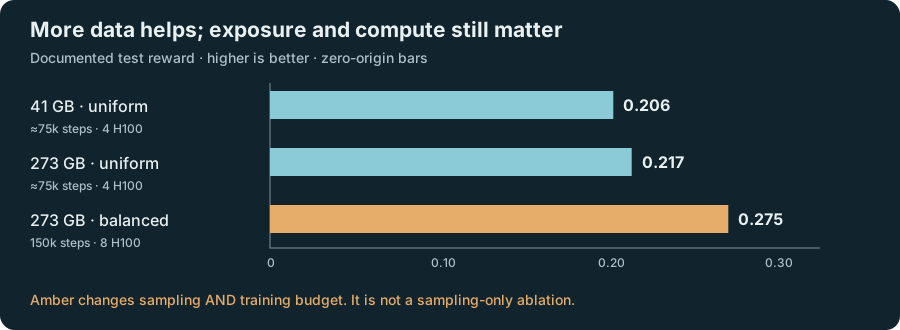
Expanding the corpus under the same model and uniform-sampling setup raises reward from about 0.206 to 0.217. The balanced recipe reaches 0.275, but also trains longer with more hardware. Its larger improvement cannot be credited to sampling alone.
The final run also shows diminishing returns: an earlier model scores about 0.274. These comparisons helped select the recipe and included test results, so they are development evidence rather than independent confirmation. Repeated runs and a fresh held-out comparison would strengthen the conclusion.
Detailed results
| Corpus / sampling | Schedule / hardware | Test reward |
|---|---|---|
| 41 GB / uniform | ≈75k steps; 4 H100 | 0.206 |
| 273 GB / uniform | ≈75k steps; 4 H100 | 0.217 |
| 273 GB / balanced | 150k steps; 8 H100 | 0.275 |
Compute and resources
Training and test inference
Reported measurement
- Time
- ≈3 h 25 min
- Hardware
- 8 × H100 training; 1 × H100 test inference
- GPU allocation
- Not separately reported for all stages
Reported stages for the reference model.
Elapsed time by stage
- Training and validation
- 194 min
- Test inference
- 11 min
Training includes 30 validation passes. Data preparation and the broader research search are excluded; corpus packing is listed in Resource details.
Timing and hardware details
Training and validation
Reported measurement
- Time
- 3 h 14 min
- Hardware
- 8 × H100
- GPU allocation
- ≈25.9 GPU-h
Includes 30 validation passes.
Corpus preparation and the wider research search are excluded.
Test inference
Reported measurement
- Time
- 11 min
- Hardware
- 1 × H100
- GPU allocation
- Not separately reported
Forecasts all 97 evaluation configurations.
Resource details
- Training corpus
- 273 GBReported corpus size. Packing it took 17 minutes on the training host.
Find out which information is missing
Longer history may help a model identify slow cycles; jointly modeling several variables may help it connect related signals. Neither is an established fix here. Compare one change at a time with the same data and computation, then inspect short and long horizons separately. For uncertainty, check how often observations actually fall inside the forecast ranges across many series.
References and provenance
GIFT-Eval: A Benchmark For General Time Series Forecasting Model Evaluation
Introduces the broad forecasting benchmark and its official evaluation tools.
TimesFM
Provides the architecture code behind the reference model; this task trains its own smaller configuration from random weights.
Task definition and experimental evidence
Defines the permitted training data, held-out forecasting series and scoring rules for this environment.
Code links require access to the project’s GitHub repository.
Leaderboard
SimulatedDesign preview · leaderboard values and research histories are simulated.
| # | Method | Type | Forecast reward ↑ | Relative MASE ↓ | Relative WQL ↓ | Research time | Run |
|---|---|---|---|---|---|---|---|
| 1 | Agent search | 0.6242 | 0.4668 | 0.3025 | 76 h | ||
| 2 | Agent search | 0.6225 | 0.4681 | 0.3044 | 60 h | ||
| 3 | TimesFM-3 (50.9M, from scratch) | Reference | 0.6200 | 0.4700 | 0.3072 | — | — |
| 4 | Seasonal Naive | Reference | 0.5084 | 0.5732 | 0.4216 | — | — |
How to read these leaderboard metrics
These leaderboard values and research histories are simulated design examples. The leaderboard is ranked by Forecast reward. The research curves show relative improvement in this metric over TimesFM-3 (50.9M, from scratch); only accepted new-best results update the retained trajectory. A positive gain means a better result, with the sign adjusted for metrics where lower is better. The task protocol is described in Task & evaluation above. These preview columns and trajectories are not measured benchmark results and must not be compared with the recorded experiments. The leaderboard and search curves below are simulated interface examples, not measured experiments—even rows named after real baselines. Their illustrative component metrics obey the reward formula but do not describe those models. Use the evidence tables for measured rewards: Seasonal Naive 0.0075 and the 50.9M scratch baseline 0.275.
- Forecast rewardPrimary metric · Higher is better
- The task-specific aggregate forecast score. Its component metrics, reference normalization and evaluation horizon determine how improvements should be interpreted.
- Relative MASELower is better
- Mean absolute scaled error relative to the task’s comparison forecaster. Keep the seasonal scaling and reference denominator fixed across methods.
- Relative WQLLower is better
- Weighted quantile loss relative to the protocol’s reference forecaster, measuring probabilistic quantile-prediction quality.
AI4AI research progress
Research trajectory
Runtime–performance frontier
How improvement is measured
Relative improvement over TimesFM-3 (50.9M, from scratch) in the primary metric; only retained results update the best-so-far curve.
Accepted new-best experiments raise the trajectory. The frontier includes evaluated candidates; trial, partial and stopped experiments are excluded.