
Surface Code Decoding
Decode logical information from repeated quantum measurements.
Task & evaluation
- Objective
- Recover a quantum memory from noisy measurement clues.
- Input
- Detection events over time and the arrangement of checks.
- Output
- The probability that the stored logical answer flipped.
- Data
- About 2.6 million training experiments and 666,000 validation experiments.
- Evaluation
- Accuracy balanced across the two code sizes and experimental conditions.
- Research challenge
- Resolve ambiguous error histories while making decisions efficiently.
Understanding the task
See why noisy error clues can support different explanations, and how a decoder learns to protect a quantum memory.
Recovering a quantum memory from noisy clues
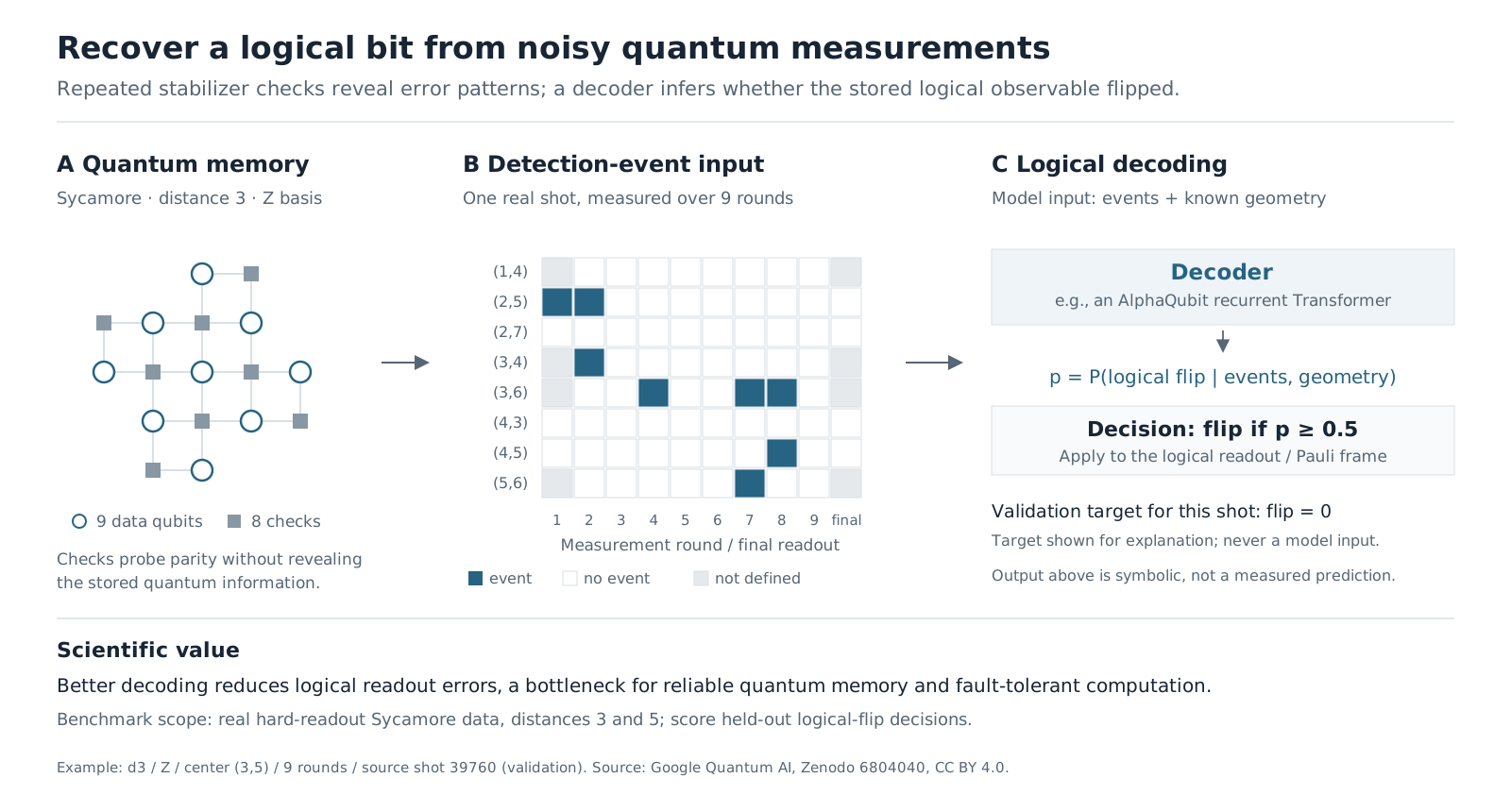
A quantum memory spreads information across several physical qubits because each qubit is fragile. Repeated parity checks reveal patterns associated with errors without directly reading the stored logical information. A decoder interprets those patterns to decide whether the final logical answer has flipped.
The clues are ambiguous. A detection event is a change in a check, not a picture of the faulty qubit. Several hidden chains of faults can produce the same endpoints but have different logical consequences. The interactive strip shows why joining the nearest clues is not always the whole problem.
Same syndrome. Different logical outcome.
Explore a five-qubit repetition strip: one error type, four parity checks, two absorbing boundaries. It illustrates the chain and boundary logic of surface-code decoding, without reproducing a Sycamore patch or its noise model.
1 · Endpoints do not specify a chain
The local correction cancels the data error.
2 · Repeated checks add a time axis
A data error produces two detections in the same round.
Try this: switch to the boundary correction, then combine both faults in the history. A decoder must infer a logical class from noisy endpoints in space and time; the hidden fault chains are shown here only to explain the mechanism.
How the real task differs
The benchmark uses distance 3 and 5 surface codes, X/Z memory bases, and odd round counts 1–25. Inputs are packed detection events, ideal circuits and sample IDs. Return the probability of the official logical-path observable flip; the decision is p ≥ 0.5. These controls do not simulate hardware or compute benchmark accuracy.
Official P = 1 − balanced logical failure: average over round counts, then geometry/basis groups, then equally over the two distances. The reward linearly maps two fixed reference accuracies (approximately 0.7160 and 0.7615) to 0 and 1, clipping outside that range; the scorer uses the full-precision constants. The toy residual parity above is separate from this scorer.
A real public hardware input
Inside one independent AlphaQubit specialist
An independently trained model reads how error clues evolve over time
- Read the observationsCombine detection events with the locations of checks
- Embed each checkRepresent what each check observed and where it sits
- Update the memoryConnect current spatial clues with information remembered from earlier rounds
- Read the terminal stateCombine the final evidence to estimate whether the logical answer flipped
- Make a decisionPredict a flip when its probability is at least one half
The recurrence carries information between rounds; attention combines spatial evidence within a round. The hidden physical fault history is never supplied. Training teaches the model which histories are associated with logical errors.
Why balancing changes the answer
Illustrative calculator: choose the mean failure after averaging each distance’s durations and geometry/basis groups. These sliders do not run a decoder.
Official balanced P0.75000
Clipped reward0.74673
Pooled accuracy (not the score)0.78000
Equal weighting gives both distances half the score; pooling would give d3 four times the influence.
P = 1 − (d3 failure + d5 failure) / 2. Reward rescales P between the two reference decoders, with values limited to 0–1. Try reducing only d5 error: the equal-distance score rewards that improvement more than pooled accuracy does.
Real hardware histories
The task uses Sycamore experiments with two surface-code sizes, called distances three and five. They have nine and twenty-five data qubits respectively. Larger distance adds redundancy, but also introduces more noisy operations; better protection must be measured rather than assumed.
Examples contain detection events across one to twenty-five measurement rounds, along with circuit geometry. About 2.6 million shots train the model and 666,000 support validation. A shot is one complete memory experiment. The decoder predicts a flip probability; it does not receive the hidden fault history.
The historical test uses separate shots, but is publicly available upstream. Models must learn from the allowed data rather than recover released answers. Simulation noise models use development check measurements, including validation measurements, but not validation logical labels or test shots.
Technical details
| Partition | Shots per condition | All 130 conditions | Use |
|---|---|---|---|
| Train | 19,880 | 2,584,400 | Fit model parameters; even source shots |
| Validation | 5,120 | 665,600 | Select checkpoints; remaining even shots |
| Historical test | 25,000 | 3,250,000 | Final score only; odd source shots |
Give both code sizes a fair voice
The primary score is one minus the logical failure rate, averaged across durations and geometry groups and then equally across the two code distances. Equal weighting prevents the more numerous distance-three conditions from dominating.
If the two distances have failure rates 20% and 30%, the balanced accuracy is 75%. Pooling all shots would instead give 78% because there are four times as many distance-three conditions. A normalized reward rescales balanced accuracy between matching and tensor-network reference decoders; reward one does not mean error-free memory.
Technical details
| Quantity | Calculation | Meaning |
|---|---|---|
| d3 mean failure | 0.20 | Mean after averaging durations and eight groups |
| d5 mean failure | 0.30 | Mean after averaging durations and two groups |
| Balanced failure | (0.20 + 0.30) / 2 = 0.25 | Each distance receives half the weight |
| Primary P | 1 − 0.25 = 0.75 | Compare predictions at p ≥ 0.5 |
| Reward | (0.75 − 0.7160463462) / 0.0454696154 ≈ 0.7467 | Then clip to [0,1] |
Remembering how the clues develop
The AlphaQubit-inspired reference maintains a learned state for each check. At every round it combines new events with its memory of earlier rounds. Attention lets it connect spatially separated clues, while recurrent memory tracks their evolution through time.
The final state produces a probability that the logical observable flipped. Ten specialists cover different geometries and memory bases. This is an independent reconstruction of the published approach, not released Google code or weights.
Only discrete detection events and ideal geometry are available here. Richer analogue readouts and information about leakage outside the intended qubit states are excluded, so the task is narrower than the original paper’s full setting.
Why start with simulation?
Simulations cheaply generate many labeled fault histories. They teach a model recurring patterns before adaptation to real hardware examples. Hardware adaptation can then address behavior the simulator misses.
Training rewards probabilities that agree with the logical labels, and adds a smaller task of predicting later check measurements. That auxiliary task encourages the internal memory to carry useful temporal information. It is a plausible mechanism, not proof that a particular noise process explains the measured improvement.
Technical details
| Predicted flip p | Logical BCE = −ln(p) | Threshold decision |
|---|---|---|
| 0.10 | 2.303 | Incorrect |
| 0.40 | 0.916 | Still incorrect |
| 0.80 | 0.223 | Correct |
Better decoding, with an important unresolved weakness
The independent trained model reaches about 75.6% balanced accuracy, compared with 71.6% for the matching reference and 76.2% for released tensor-network predictions on the same shots. These comparisons locate performance within this dataset, not the full literature.
A separate reference run has fitted error rates of about 3.0% per round at distance three and 3.2% at distance five. The larger code does not improve this diagnostic. An aggregate accuracy can therefore conceal the central question of whether adding qubits actually improves protection.
These runs do not establish robustness across training seeds or changing hardware noise. The published Nature results also use different folds and ensembles, so comparable headline numbers would not establish equivalent performance.
| Decoder | Primary P | Normalized reward |
|---|---|---|
| Matching reference | 0.716 | 0 |
| AlphaQubit reference | 0.755 | 0.858 |
| Independent AlphaQubit training | 0.756 | 0.872 |
| Released tensor-network predictions | 0.762 | 1 |
Compute and resources
Reference training and testing
Reported measurement
- Time
- Not separately reported
- Hardware
- RTX PRO 6000 Blackwell Max-Q
- GPU allocation
- ≈200.3 GPU-h
Recorded allocation for simulation pretraining, adaptation to hardware data and testing.
GPU allocation by stage
- Simulation pretraining
- 179.963 GPU-h
- Hardware adaptation
- 19.9467 GPU-h
- Test inference
- 0.3911 GPU-h
Actual card-hours; not H200-equivalent compute. Earlier model-development campaigns are excluded.
Resource details
- Parallel allocation
- Up to 8 GPUsMaximum simultaneous GPU count in the recorded campaign; GPU-hours are not wall-clock hours.
- Distance-3 / distance-5 peak GPU memory
- 9.61 / 24.46 GBOptimizer probes on RTX PRO 6000 Blackwell Max-Q, BF16, batch 256, 25 rounds. These are not streaming latency measurements.
Where does the memory fail?
Break down errors by experiment duration, geometry and code size. Improvements confined to short histories may leave long-lived memory unchanged. Better simulation, longer-memory models or hybrid neural and matching methods could help; each should be tested for both accuracy and the time needed to update after one new round.
References and provenance
AlphaQubit: recurrent Transformer decoding
Explains how a learned decoder can infer logical errors from repeated quantum error-correction measurements.
Sycamore surface-code dataset
Supplies public quantum-device measurements, including the real validation example shown on this page.
Task definition and experimental evidence
Defines the restricted inputs and balanced evaluation used in this release, alongside the reproduction results.
Code links require access to the project’s GitHub repository.
Leaderboard
SimulatedDesign preview · leaderboard values and research histories are simulated.
| # | Method | Type | Decoder reward ↑ | Balanced performance P ↑ | Balanced logical failure ↓ | Research time | Run |
|---|---|---|---|---|---|---|---|
| 1 | Agent search | 0.7305 | 0.7493 | 0.2507 | 76 h | ||
| 2 | Agent search | 0.7275 | 0.7491 | 0.2509 | 60 h | ||
| 3 | AlphaQubit (independent reproduction) | Reference | 0.7250 | 0.7490 | 0.2510 | — | — |
| 4 | QRENND | Reference | 0.5945 | 0.7431 | 0.2569 | — | — |
How to read these leaderboard metrics
These leaderboard values and research histories are simulated design examples. The leaderboard is ranked by Decoder reward. The research curves show relative improvement in this metric over AlphaQubit (independent reproduction); only accepted new-best results update the retained trajectory. A positive gain means a better result, with the sign adjusted for metrics where lower is better. The task protocol is described in Task & evaluation above. These preview columns and trajectories are not measured benchmark results and must not be compared with the recorded experiments. The simulated preview columns obey the official relationship between balanced P, failure and reward. They are design examples, not the measured H100 or frozen Blackwell experiments reported above; the search trajectories are also simulated.
- Decoder rewardPrimary metric · Higher is better
- The task’s normalized quantum-decoding performance score. Its reference anchors are defined by the scoring protocol.
- Balanced performance PHigher is better
- One minus logical failure averaged over durations, then groups, then equally over d3 and d5.
- Balanced logical failureLower is better
- One minus balanced P; shot-level failure, not fitted logical error per round.
AI4AI research progress
Research trajectory
Runtime–performance frontier
How improvement is measured
Relative improvement over AlphaQubit (independent reproduction) in the primary metric; only retained results update the best-so-far curve.
Accepted new-best experiments raise the trajectory. The frontier includes evaluated candidates; trial, partial and stopped experiments are excluded.