
PDE Surrogate
Learn dynamics that transfer across physical systems.
Task & evaluation
- Objective
- Learn one model that predicts how different physical systems evolve.
- Input
- Initial physical fields and boundary conditions.
- Output
- Continuing physical fields without seeing future observations.
- Data
- Sixteen source datasets and three transfer datasets with declared training and validation pools; 1,085 held-out trajectories.
- Evaluation
- Prediction error relative to each field’s spatial variation, across four equally weighted groups.
- Research challenge
- Prevent small errors from growing while handling different equations and fields.
Understanding the task
Can one model learn how many different physical systems evolve? This task asks it to continue moving fields from a few observed frames, preserving useful structure as its own errors accumulate.
Predict motion without solving every equation
A numerical solver follows physical equations to advance a fluid or another evolving field. A learned surrogate tries to infer that evolution from examples. If accurate enough, it could make repeated simulations and parameter searches much faster.
Here one model sees four initial frames and predicts what comes next across sixteen equation families and three additional datasets. The systems include flowing fluids, active particles and layers of gas that mix while cooling. Their fields, boundaries and grids differ. A smooth-looking prediction can still erase a vortex or miss the mixing that scientists care about.
Watch a small model error become a rollout error
Synthetic periodic advection–diffusion, one channel on a 24 × 24 grid. This analytic teaching example is not a benchmark result or a trained model.
Fixed field scale: −1.5 (blue) → 0 (dark) → +1.5 (amber); extreme colors saturate.
The vertical marker follows the selected step. The solid curve feeds predictions back in; the dashed curve resets to truth every step. Teacher forcing is a diagnostic, not the benchmark inference setting.
Try this: increase bias and advance the forecast. Then select “Nearly uniform field”: a small absolute offset can overwhelm the remaining spatial variation. A spatial-mean prediction also looks smooth but loses all structure (VRMSE ≈ 1 for a varying field).
Equations behind this illustration
The toy truth is u(x,y,t) = A exp(−0.025t) [sin(x − 0.12t) + 0.4 cos(y − 0.08t)] on a periodic square. It solves a constant-coefficient advection–diffusion equation. The toy prediction adds phase bias b and a uniform offset 0.2b each step. Free rollout accumulates both over t steps; teacher forcing applies them once to the true previous field. This simplified one-frame update illustrates feedback; the real model receives four initial 2D frames plus metadata.
Plots compute spatial mean squared error and unbiased target variance over 576 cells. VRMSE = √[MSE / (variance + 10⁻⁷)], capped at 10, per channel and predicted step. Real horizons are 26 steps for the equation corpus, 30 for The Well and 10 for PDEArena; this toy displays 30 for comparison. Actual scores average steps, channels and cases, then map each of four group means through R(v) = clip((1 − log₁₀(max(v, 0.01))) / 3, 0, 1) and average the four rewards equally. No aggregate benchmark reward is inferred from this single toy field.
Sources: Task specification · Metric and inference contract.
Two real physical systems, one required interface
Public upstream visualizations from The Well. These animations illustrate simulated physics; they are not this track’s held-out inputs or predictions. External images require access to the source host.
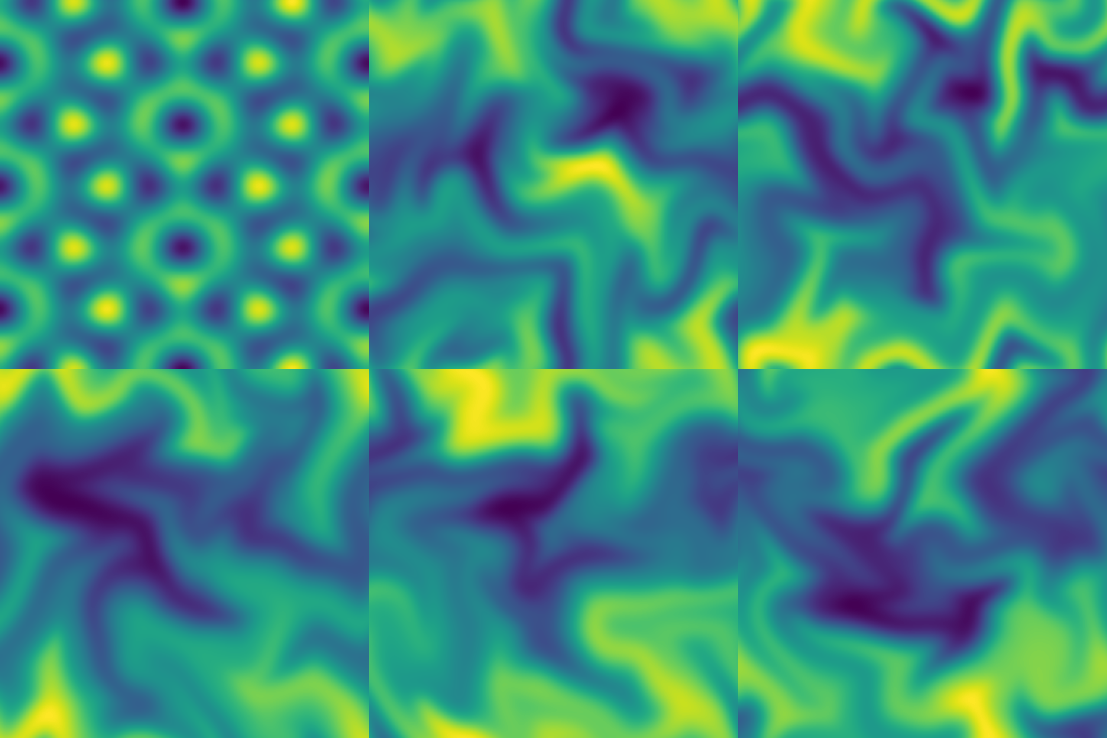
Motion of active particles couples to fluid flow and orientation. The scored case includes 11 channels, so this scalar view shows only part of the state.
Animation and dataset
Hot and cold gas mix as cooling changes the fluid. Density, pressure and both velocity components must be predicted on a rectangular grid.
Animation and datasetVisualizations: The Well / Polymathic AI, served by Flatiron Institute. Dataset license: CC BY 4.0. Each animation uses its source’s own scale; colors are not comparable between systems.
Follow one forecast through the model
4 × C × X × Y
Four observed frames, with information about the domain and its boundaries.Training statistics
The reference z-scores its fields. No statistics from future target frames.ConvNeXt U-Net
Combine broad spatial patterns with fine detail.Advance context
Return to physical units; use the predicted fields to continue without future truth.This is the PDEArena reference. It learns from compatible three-channel fields and repeats the last frame for other channel counts; a fully shared model remains the goal.
Why four group scores matter
Move one group’s mean error while holding the others fixed. This is a scoring calculator with illustrative values, not an experiment. The corpus contains many datasets but receives the same final weight as each transfer group.
R(v) = clip((1 − log₁₀(max(v, 0.01))) / 3, 0, 1). Improving any one group from 1 to 0.1 raises total reward by 1/12 ≈ 0.0833, regardless of its trajectory count. Changing only the corpus cannot erase failures in the other three groups.
Different fields describe different physics
For a simple fluid, the state may include a scalar field and two velocity components. Active matter also tracks particle orientation, producing eleven scored channels. The radiative layer includes density, pressure and velocity on a rectangular grid. These are physical quantities, not image color channels.
Trajectories are separated into training, validation and evaluation sets. Models start from random weights and see only initial frames and metadata during evaluation. The additional datasets are part of the declared learning setup, so “transfer” does not automatically mean predicting a wholly unseen kind of physics.
Technical details
| Source | Channels and grid | Predicted frames | What changes |
|---|---|---|---|
| Equation corpus | 1–multiple channels; 256 × 256 | 4–29 (26) | Sixteen equation families; varying constants |
| PDEArena Navier–Stokes | Scalar u, velocity vx/vy; 3 × 128 × 128 | 4–13 (10) | Wall boundaries; scalar and velocity dynamics |
| The Well: active matter | Concentration + velocity + two tensors; 11 × 256 × 256 | 4–33 (30) | Periodic boundaries; coupled scalar/vector/tensor fields |
| The Well: radiative layer | Density, pressure, velocity; 4 × 128 × 384 | 4–33 (30) | Anisotropic domain; mixing and cooling |
Measure mistakes against the structure of the field
The main error is variance-normalized root mean squared error, or VRMSE. It compares prediction error with how much the true field varies across space. This allows fields with different units and amplitudes to be compared. A nearly uniform field makes even a small absolute mistake important relative to its remaining structure.
The equation corpus and each of the three additional datasets contribute equally after a logarithmic score mapping. Group errors of 1 and 0.1 give rewards of about 0.33 and 0.67. Reducing error by a factor of ten matters wherever it occurs; strong performance on one group cannot completely hide failure on another.
Feed predictions back into the next step
The reference uses an encoder–decoder network: compress spatial patterns, combine information at different scales, then reconstruct the next field. Connections between corresponding scales help retain fine detail. The inputs are normalized using training data and outputs return to physical units.
To continue a trajectory, the model must use its own predicted fields as context. This creates a mismatch with training examples that always start from the truth. A tiny phase error can shift a vortex, alter the next prediction and grow over time. The interactive example lets you compare this accumulation with repeatedly restarting from the true field.
A specialist is a starting point for a shared model
The reference is trained on PDEArena fluid data. It uses its learned network on compatible three-channel inputs and otherwise repeats the last observed field, a simple strategy called persistence. Its overall reward therefore does not establish a universal solution.
Longer training reduces PDEArena error from about 0.297 to 0.282, while overall reward moves only from 0.345 to 0.347. The small overall gain makes sense: the other groups largely retain the same behavior. Repeating this experiment with multiple training runs would help establish how reliable the change is.
| Predictor | Reward | Interpretation |
|---|---|---|
| Persistence | 0.283 | Keep the last observed field |
| Last-frame spatial mean | 0.310 | Discard spatial structure |
| Small starter | 0.313 | Basic learned pipeline |
| CNextU-net reference | 0.345 | PDEArena-trained model with fallback |
| CNextU-net, longer training | 0.347 | Same specialized model; selected by validation |
Look where the model is actually learning
The reference’s error is about 0.30 on its training domain, compared with 1.52 on active matter and 1.36 on the radiative layer, where it uses persistence. This breakdown identifies a concrete gap: learning to represent different physical fields, rather than improving an already specialized fluid predictor alone.
Detailed results
| Group | Mean VRMSE ↓ | Group reward ↑ | Inference behavior |
|---|---|---|---|
| Corpus (16 families) | 1.188 | 0.308 | Learned model for compatible 3-channel cases; persistence otherwise |
| PDEArena Navier–Stokes | 0.297 | 0.509 | Training domain of the learned model |
| Active matter | 1.523 | 0.272 | Persistence |
| Radiative layer | 1.358 | 0.289 | Persistence |
Compute and resources
Reference training
Reported measurement
- Time
- ≈10 h
- Hardware
- 1 × H100
- GPU allocation
- Not separately reported
Reported training of the reference model.
Elapsed time by stage
- Training
- 10 h
Only training is timed; evaluation and preparation are unreported.
Evaluation and data preparation are additional; no numerical-solver speedup was measured.
Separate unstable forecasts from unfamiliar physics
Plotting error over time can reveal two different problems. A model that begins accurately but drifts may need training on longer self-generated trajectories. A model that fails immediately on orientation or pressure fields may need a better shared representation. Testing those changes separately, with the same data and computation, would make an improvement easier to explain.
References and provenance
The Well: a Large-Scale Collection of Diverse Physics Simulations for Machine Learning
Provides diverse simulated systems, including the active matter and radiative mixing examples used to explain the task.
PDE-Transformer: Efficient and Versatile Transformers for Physics Simulations
Studies a general-purpose model architecture for learning physical evolution on regular grids.
Task definition and experimental evidence
Defines the task’s prediction targets and scoring setup, with documentation of the specialized reference model.
Code links require access to the project’s GitHub repository.
Leaderboard
SimulatedDesign preview · leaderboard values and research histories are simulated.
| # | Method | Type | Rollout reward ↑ | VRMSE ↓ | Transfer VRMSE ↓ | Research time | Run |
|---|---|---|---|---|---|---|---|
| 1 | Agent search | 0.5885 | 0.5417 | 0.7008 | 76 h | ||
| 2 | Agent search | 0.5870 | 0.5431 | 0.7025 | 60 h | ||
| 3 | CNextU-net (simulated reference) | Reference | 0.5850 | 0.5450 | 0.7050 | — | — |
| 4 | Channel-shared U-Net | Reference | 0.4797 | 0.6646 | 0.8598 | — | — |
How to read these leaderboard metrics
These leaderboard values and research histories are simulated design examples. The leaderboard is ranked by Rollout reward. The research curves show relative improvement in this metric over CNextU-net (simulated reference); only accepted new-best results update the retained trajectory. A positive gain means a better result, with the sign adjusted for metrics where lower is better. The task protocol is described in Task & evaluation above. These preview columns and trajectories are not measured benchmark results and must not be compared with the recorded experiments. The leaderboard and search histories are simulated UI examples, not measured experiments. The recorded CNextU-net reference scores 0.3447 (epoch 120) or 0.3466 (best of 200 epochs), documented below. Ranking averages four log-mapped group errors; a single overall or transfer VRMSE cannot reconstruct reward. Transfer here has declared training pools and does not imply zero-shot evaluation.
- Rollout rewardPrimary metric · Higher is better
- The task-defined score for predicted physical trajectories over the evaluation rollout, rather than only the next simulation step.
- VRMSELower is better
- Variance-normalized root mean squared error between predicted and reference physical fields, aggregated as specified by the task.
- Transfer VRMSELower is better
- Illustrative transfer aggregate in this simulated table. The real scorer treats PDEArena, active matter and radiative layer as three separate, equally weighted groups alongside the corpus.
AI4AI research progress
Research trajectory
Runtime–performance frontier
How improvement is measured
Simulated relative improvement over the illustrated CNextU-net reference; only retained examples update the curve. Not an empirical search history.
Accepted new-best experiments raise the trajectory. The frontier includes evaluated candidates; trial, partial and stopped experiments are excluded.